


About ARIMA Model
ARIMA stands for Autoregressive Integrated Moving Average and it's a technique for time series analysis and forecasting possible future values of a time series. It is especially effective for data that changes over time in a trend or seasonal pattern.
For our project in Pandi, Bulacan, ARIMA is used to forecast waste generation using historical data. Specifically, the system utilizes the ARIMA(1,1,1) model configuration, which was identified as the most suitable based on the dataset’s trend and behavior.
The term “ARIMA” comes from three key components:
- AR (AutoRegressive) – uses the relationship between current and previous values.
- I (Integrated) – makes the data stationary by removing trends and seasonality.
- MA (Moving Average) – uses past forecast errors to improve predictions.

Purpose
ARIMA (AutoRegressive Integrated Moving Average) is a forecasting model that predicts future waste generation based on past yearly data. Since waste is closely linked to population growth, ARIMA helps estimate how much waste will be produced in the coming years.

Why it Matters?
- Waste generation usually grows as the population increases.
- Forecasting allows cities and communities to prepare in advance.
- Provides a scientific, data-based way to avoid waste overflows and lack of facilities.
- Helps decision-makers design better waste management strategies.

Benefits
- Predicts long-term waste trends accurately.
- Shows the link between population growth and waste generation.
- Helps plan budgets for trucks, bins, recycling centers, and landfills.
- Useful for checking if waste reduction programs are effective.
- Supports sustainability goals and environmental protection.
Specifying ARIMA Components
ARIMA stands for AutoRegressive Integrated Moving Average, and it works by combining three core elements. Each component plays a unique role in identifying and forecasting patterns in time series data.
p: the order of the Autoregressive part of ARIMA
d: the degree of differencing involved
q: the order of the Moving Average part
- AR (AutoRegressive)
Uses the relationship between a value and its past values. - I (Integrated)
Makes the data stationary by differencing to remove trend/seasonality. - MA (Moving Average)
Relates a value to past forecast errors to improve predictions.
About Linear Regression
Linear Regression predicts a dependent variable from an independent variable by fitting a best-fit straight line.
For our project in Pandi, Bulacan, Linear Regression is used to forecast population growth using historical population data.
Purpose
Linear Regression predicts future values by analyzing the relationship between two variables—key to estimating population growth trends that influence waste generation.
Why it Matters?
- Population growth drives waste generation.
- Forecasting population prepares planners for future needs.
- Data-driven approach beats guesswork.
- Supports planning for infrastructure and services.
Benefits
- Simple, interpretable model with one predictor.
- Visualizes trend with a straight line.
- Connects population and waste forecasting.
- Supports sustainable planning.
Linear Regression Formula
The formula shows how the dependent variable changes given the independent variable.
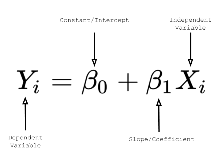
Where:
- yᵢ – predicted value.
- β₀ – intercept.
- β₁ – slope.
- xᵢ – independent variable.
About MAE Validation Metric
Mean Absolute Error (MAE) measures the average size of prediction errors (ignores direction).
For this project, a lower MAE means ARIMA/MLR predictions are closer to reality.
Formula:
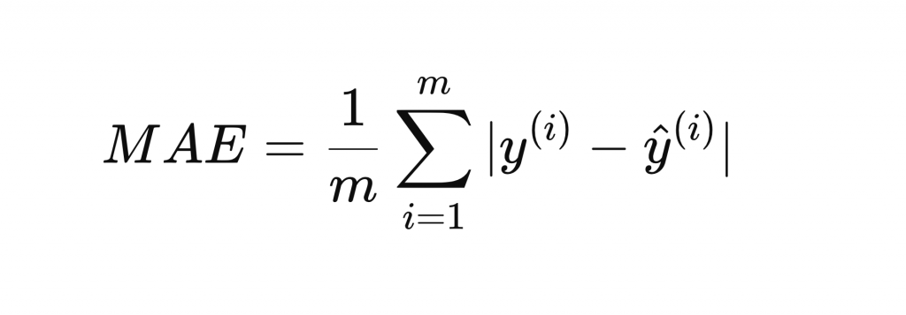
Where:
- n – number of observations.
- yᵢ – actual.
- ŷᵢ – predicted.
- |·| – absolute value.
Purpose
Shows average difference between predictions and actuals.
Why it Matters?
- Explains forecast accuracy in simple terms.
- Lower MAE = better model.

How it Works?
- Compute |yᵢ − ŷᵢ| for each point.
- Average them.
Example:
- (1000→1050) error=50; (1200→1180) error=20 ⇒ MAE=(50+20)/2=35
Benefits
- Easy to interpret.
- Same unit as data.
- Good for comparing models.
About RMSE Validation Metric
Root Mean Squared Error (RMSE) penalizes large errors more strongly (squaring).
Lower RMSE means forecasts are closer to actuals—useful when big mistakes are costly.
Formula:
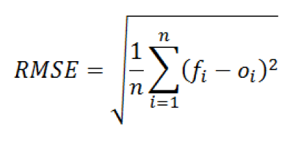
Where:
- n – observations.
- yᵢ – actual.
- ŷᵢ – predicted.
- (yᵢ − ŷᵢ)² – squared error.
Purpose
Captures error magnitude; emphasizes large misses.
Why it Matters?
- Highlights costly mistakes.
- Complements MAE.
How it Works?
- Square errors, average, then square-root.
Example: errors 50 & 20 ⇒ mean of squares 1450 ⇒ RMSE ≈ 38.08
Benefits
- Penalizes big errors.
- Same unit as data.
- Great for model comparison.
About R² Validation Metric
R² explains how much variance in actual data is explained by the model.
Formula:
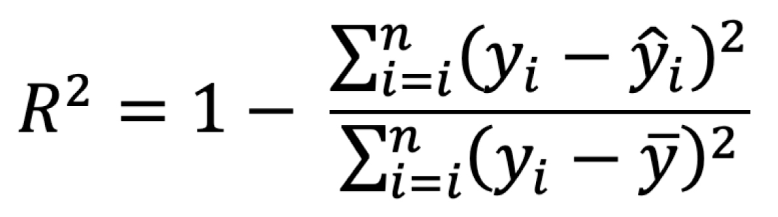
Where:
- yᵢ – actual, ŷᵢ – predicted, ȳ – mean.
Purpose
Measures goodness of fit (0 to 1).
Why it Matters?
- Easy “percentage-like” understanding.
- Higher R² → better fit.
How it Works?
Compares predictions against the mean baseline.
- R²=0.85 → explains 85% of variation.
Benefits
- Quick “at a glance” accuracy.
- Complements MAE/RMSE.
About Methodology for Analytics Modeling
CRISP-DM is a structured, 6-phase approach for analytics projects.
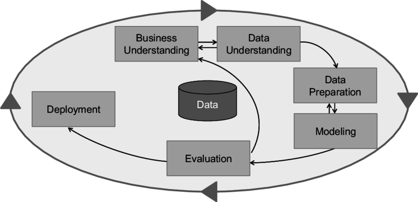
CRISP-DM Framework:
- Business Understanding – Objectives & requirements.
- Data Understanding – Collect initial data.
- Data Preparation – Clean & format.
- Modeling – Build forecasts.
- Evaluation – Check against goals.
- Deployment – Use results for decisions.
Purpose
Gives a repeatable framework aligned to MENRO goals.
Why it Matters?
- Prevents ad-hoc analysis.
- Makes work transparent & reproducible.
How it Works?
Cycle through BU → DU → DP → Modeling → Eval → Deploy.
Benefits
- Clear roadmap.
- Adaptable to data changes.
- Supports sustainable planning.